
Overview of AQA A-level Mathematics qualifications
Subject content:
1. Overarching themes
| Syllabus component | Content |
|---|---|
| Mathematical argument, language and proof | • Construct and present arguments using diagrams, graph sketching, logical deduction, and precise language with correct symbols (e.g., constant, coefficient, expression, equation, function, identity, index, term, variable). • Understand and use mathematical language and syntax. • Use set theory language and symbols, applying them to inequalities and probability. • Understand functions, including their domain and range. • Comprehend and critique mathematical arguments, proofs, and justifications. |
| Mathematical problem solving | • Identify mathematical structures in situations and simplify them for problem-solving. • Solve unstructured and contextual problems through extended arguments. • Communicate solutions within their original context. • Use numerical methods when analytical solutions are unavailable. • Assess the accuracy and limitations of solutions. • Follow the problem-solving cycle: specify, collect, process, represent, and interpret data. • Use diagrams for extracting information and solving problems, including mechanics. |
| Mathematical modelling | • Convert real-world situations into mathematical models with assumptions. • Apply models to explore situations using suitable inputs. • Interpret model outputs in the original context. • Refine models by evaluating outputs and assumptions. • Understand and use modeling assumptions effectively. |
2. Proof
• Understand mathematical proof structure, progressing logically from assumptions to conclusions.
• Use deduction, exhaustion, and contradiction for proofs.
• Disprove with counterexamples.
• Apply contradiction to prove the irrationality of √2, the infinity of primes, and unfamiliar proofs.
3. Algebra and functions
• Understand and apply laws of indices for rational exponents.
• Manipulate surds and rationalize denominators.
• Analyze quadratic functions: discriminant, completing the square, solving equations.
• Solve linear and quadratic simultaneous equations.
• Solve and graphically interpret linear/quadratic inequalities, using set notation.
• Manipulate polynomials: factorize, divide, simplify expressions, use the factor theorem.
• Work with function graphs: sketch and interpret, understand proportional relationships.
• Use composite and inverse functions, including graphing.
• Apply transformations to y = f(x) and sketch transformed graphs.
• Decompose rational functions into partial fractions.
• Use functions in modeling, considering limitations and refinements.
4. Coordinate geometry in the (x,y) plane
• Use straight line equations y − y1=m (x − x1) and ax + by + c = 0; conditions for parallel/perpendicular lines; apply in various contexts.
• Understand circle geometry: equation (x − a)2 + (y − b)2 = r2; find center/radius by completing the square; properties:
– Right angle in a semicircle;
– Perpendicular from center bisects chord;
– Radius perpendicular to tangent at the circle.
• Use and convert parametric equations of curves between Cartesian and parametric forms.
• Apply parametric equations in various modeling contexts.
5. Sequences and series
• Use binomial expansion (a + bx)n for positive integer n; notations n!, nCr and ![]() ; link to binomial probabilities; extend to any rational n for approximation, valid for
; link to binomial probabilities; extend to any rational n for approximation, valid for ![]() < 1.
< 1.
• Work with sequences given by a formula for the nnnth term or generated by xn+1 = f(xn); identify increasing, decreasing, and periodic sequences.
• Understand and use sigma notation for sums of series.
• Understand and work with arithmetic sequences and series, including formulae for the n th term and sum to n terms.
• Understand and work with geometric sequences and series, including formulae for the nnnth term, sum of a finite geometric series, and sum to infinity of a convergent geometric series |r| < 1.
• Use sequences and series in modeling.
6. Trigonometry
• Understand and use sine, cosine, tangent definitions; sine/cosine rules; triangle area formula ![]() ; radian measure for arc length/sector area.
; radian measure for arc length/sector area.
• Small angle approximations: sinθ ≈ θ, cosθ ≈ 1 − ![]() , tanθ ≈ θ, where θ is in radians.
, tanθ ≈ θ, where θ is in radians.
• Sine, cosine, tangent functions: graphs, symmetries, periodicity; exact values at key angles.
• Definitions/relationships: secant, cosecant, cotangent, arcsin, arccos, arctan; graphs, ranges, domains.
• Identities: tanθ ≡ sin![]() ; sin2 θ + cos2 θ ≡ 1; sec2 θ ≡ 1 + tan2 θ and cosec2 θ ≡ 1 + cot2 θ.
; sin2 θ + cos2 θ ≡ 1; sec2 θ ≡ 1 + tan2 θ and cosec2 θ ≡ 1 + cot2 θ.
• Understand and use double angle formulae; use of formulae for sin (A ± B) , cos (A ± B) and tan (A ± B); understand geometrical proofs of these formulae.
Understand and use expressions for acos θ + bsin θ in the equivalent forms of rcos (θ ± а) or rsin (θ ± а)
• Solve trigonometric equations, including quadratic/multiple angle equations.
• Construct proofs with trigonometric functions/identities.
• Apply trigonometric functions to vectors, kinematics, and forces.
7. Exponentials and logarithms
• Know and use ax and ex functions and their graphs.
• Know that the gradient of ekx is equal to kekx and hence understand why the exponential model is suitable in many applications
• Define logax as the inverse of ax, where a is positive and x≥0; know ln x and its graph; ln x as the inverse of ex.
• Use laws of logarithms:
logax + logay ≡ loga(xy);
logax − logay ≡ loga![]() ;
;
klogax ≡ logaxk
(including, for example, k = − 1 and k = −![]() ).
).
• Solve ax = b equations.
• Use logarithmic graphs to estimate parameters in y = axn and y = kbx.
• Understand and model exponential growth/decay; apply to continuous compound interest, radioactive decay, drug concentration decay, population growth; consider limitations and refinements.
8. Differentiation
• Understand the derivative as the tangent’s gradient to y = f(x); limits; rate of change; sketching gradients; second derivatives; differentiation from first principles for small powers of x, sin x, and cos x; second derivative for gradient changes, convex/concave curves, and inflection points.
• Differentiate xn, ekx, akx, sin kx, cos kx, tan kx, ln x, and their sums/differences.
• Use differentiation for gradients, tangents, normals, extrema, stationary points, inflection points; identify increasing/decreasing functions.
• Use product, quotient, and chain rules; solve connected rates of change and inverse functions.
• Differentiate simple implicit or parametric functions.
• Create differential equations in contexts like kinematics, population growth, and price-demand models.
9. Integration
• Know and use the Fundamental Theorem of Calculus.
• Integrate xn (excluding n = −1); ekx, ![]() , sinkx, coskx; and their sums, differences, and constants.
, sinkx, coskx; and their sums, differences, and constants.
• Evaluate definite integrals for areas under and between curves.
• Understand integration as a sum limit.
• Use integration by substitution and by parts; understand these as inverses of chain and product rules.
• Integrate with partial fractions (linear denominators).
• Solve simple separable first-order differential equations, including particular solutions.
• Interpret solutions of differential equations in problem contexts, including kinematics, noting limitations.
10. Numerical methods
• Locate roots of f(x) = 0 by changes of sign in an interval; understand method failures.
• Use iterative methods and Newton-Raphson for approximate solutions; understand method failures.
• Apply numerical integration, including the trapezium rule, to estimate areas under curves.
• Solve contextual problems using numerical methods.
11. Vectors
• Use vectors in two dimensions and in three dimensions.
• Calculate and convert vector magnitude and direction.
• Perform and interpret vector addition and scalar multiplication.
• Use position vectors to calculate distances.
• Solve problems in mathematics and contexts using vectors.
12. Statistical sampling
• Use a calculator for summary statistics and standard distribution probabilities.
• Understand population and sample terms.Infer population characteristics from samples.
• Use and understand simple random and opportunity sampling methods.
• Select or critique sampling methods; recognize different samples can yield different conclusions.
13. Data presentation and interpretation
• Interpret single-variable data diagrams; histogram areas show frequency, linked to probability distributions.
• Interpret scatter diagrams and regression lines; recognize population sections; correlation ≠ causation.
• Interpret and calculate measures of central tendency, variation, and standard deviation.
• Recognize outliers; select/critique data presentation; clean data, handling missing data, errors, and outliers.
14. Probability
• Use mutually exclusive and independent events in probability; link to distributions.
• Use conditional probability with tree diagrams, Venn diagrams, two-way tables; apply the conditional probability formula. 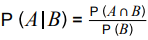
• Model with probability; critique and refine assumptions.
15. Statistical distributions
• Use discrete probability distributions, including the binomial; calculate binomial probabilities.
• Use the Normal distribution for probabilities; link to histograms, mean, standard deviation, points of inflection, and binomial distribution.
• Select suitable probability distributions with reasoning, recognizing model limitations.
16. Statistical hypothesis testing
• Understand and apply statistical hypothesis testing terms: null hypothesis, alternative hypothesis, significance level, test statistic, 1-tail test, 2-tail test, critical value, critical region, acceptance region, p-value; interpret correlation coefficients with given p-values or critical values.
• Conduct and interpret hypothesis tests for binomial distribution proportions, understanding sample inference and significance level.
• Conduct and interpret hypothesis tests for Normal distribution means with known, given, or assumed variance.
17. Quantities and units in mechanics
• Understand and use fundamental SI quantities and units: length, time, mass.
• Understand and use derived SI quantities and units: velocity, acceleration, force, weight, moment.
18. Kinematics
• Use kinematic terms: position, displacement, distance, velocity, speed, acceleration.
• Interpret kinematic graphs: displacement vs. time, velocity vs. time (gradient and area).
• Apply and derive formulas for constant acceleration in one and two dimensions.
Use calculus for kinematics: 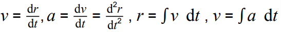 ; extend to 2 dimensions.
• Model vertical motion and projectiles using vectors.
19. Forces and Newton’s laws
• Concept of force and Newton’s first law.
• Newton’s second law: apply to straight-line motion with forces in 2D, including resolving forces.
• Weight and motion under gravity: gravitational acceleration g, its value, and dependence on location (inverse square law not required).
• Newton’s third law: equilibrium and motion in 2D, including smooth pulleys and connected particles; resolving forces and equilibrium under coplanar forces.
• Addition of forces and resultant forces; dynamics for plane motion.
• Friction: F ≤ μR, coefficient of friction, motion on rough surfaces, limiting friction, and statics.
20. Moments
• Understand and use moments in simple static contexts.
Want to learn more about Advanced Level Qualifications (A-Levels) and how they can shape your academic future? Click here to explore: A-Level Information.
Assessment
| Type of assessment | Questions | Final score | Weighting of final grade |
|---|---|---|---|
| Paper 1 | A mix of question styles, from short, single-mark questions to multi-step problems Any content from: – Proof – Algebra and functions – Coordinate geometry – Sequences and series – Trigonometry – Exponentials and logarithms – Differentiation – Integration – Numerical methods | 100 marks | 33⅓ % of A-level |
| Paper 2 | A mix of question styles, from short, single-mark questions to multi-step problems Any content from Paper 1 and content from: – Vectors – Quantities and units in mechanics – Kinematics – Forces and Newton’s laws – Moments | 100 marks | 33⅓ % of A-level |
| Paper 3 | A mix of question styles, from short, single-mark questions to multi-step problems Any content from Paper 1 and content from: – Statistical sampling – Data presentation and Interpretation – Probability – Statistical distributions – Statistical hypothesis testing | 100 marks | 33⅓ % of A-level |
Weighting of assessment objectives for A-level Mathematics
Exams will assess students on the following objectives:
AO1: Use and apply standard techniques
– Select and perform routine procedures.
– Accurately recall facts, terminology, and definitions.
AO2: Reason, interpret, and communicate mathematically
– Construct rigorous mathematical arguments and proofs.
– Make deductions and inferences.
– Assess the validity of mathematical arguments.
– Explain reasoning and use mathematical language and notation correctly.
AO3: Solve problems within mathematics and in other contexts
– Translate problems into mathematical processes.
– Interpret and evaluate solutions in context.
– Develop and use mathematical models.
– Evaluate and refine models.
| Assessment objectives AOs | Paper 1 (%) | Paper 2 (%) | Paper 3 (%) | Overall weighting (%) |
|---|---|---|---|---|
| AO1 | 50 | 50 | 50 | 50 |
| AO2 | 25 | 25 | 25 | 25 |
| AO3 | 25 | 25 | 25 | 25 |
| Total weight of components | 33⅓ | 33⅓ | 33⅓ | 100 |
Assessment weightings
The grades awarded on the papers will be scaled based on the weighting of each component. Students’ final grades will be determined by adding the scaled grades for each component. Grade boundaries will be established using this unified scale. The scale and final grades are summarized in the table below.
| Сomponent | Maximum raw mark | Scaling factor | Maximum scaled mark |
|---|---|---|---|
| Paper 1 | 100 | ×1 | 100 |
| Paper 2 | 100 | ×1 | 100 |
| Paper 3 | 100 | ×1 | 100 |
| Total scaled mark: | 300 |
If you need help with Mathematics or any other subject, our tutors are ready to support you on your academic journey. Don’t miss your chance to succeed—take a trial lesson today!


